Visualize workflows
suppressPackageStartupMessages({
    library(systemPipeR)
})
In the last section, we have learned how to run/manage workflows. In this section, we will learn advanced options how to visualize workflows.
First let’s set up the workflow using the example workflow template. For real production purposes, we recommend you to check out the complex templates over here.
dependency graph
The workflow plot is also called the dependency graph. It shows users how one step is depend on another. This is very important in SPR. A step will not be run unless all dependencies has been executed successfully.
To understand a workflow, we can simply call the sal object to print on console like so
sal
## Instance of 'SYSargsList':
##     WF Steps:
##        1. load_library --> Status: Success
##        2. export_iris --> Status: Success
##        3. gzip --> Status: Success
##            Total Files: 3 | Existing: 3 | Missing: 0
##          3.1. gzip
##              cmdlist: 3 | Success: 3
##        4. gunzip --> Status: Success
##            Total Files: 3 | Existing: 3 | Missing: 0
##          4.1. gunzip
##              cmdlist: 3 | Success: 3
##        5. stats --> Status: Success
However, when the workflow becomes very long and complex, the relation between steps are hard to see from console. Workflow plot is the useful tool to understand the workflow.
For example, the VARseq workflow is complex, we can show it by:
systemPipeRdata::genWorkenvir("varseq")
setwd("varseq")
sal <- SPRproject()
sal <- importWF(sal, file_path = "systemPipeVARseq.Rmd")
sal
## Instance of 'SYSargsList':
##     WF Steps:
##        1. load_SPR --> Status: Pending
##        2. fastq_report_pre --> Status: Pending
##        3. trimmomatic --> Status: Pending
##            Total Files: 32 | Existing: 0 | Missing: 32
##          3.1. trimmomatic-pe
##              cmdlist: 8 | Pending: 8
##        4. preprocessing --> Status: Pending
##            Total Files: 16 | Existing: 0 | Missing: 16
##          4.1. preprocessReads-pe
##              cmdlist: 8 | Pending: 8
##        5. fastq_report_pos --> Status: Pending
##        6. bwa_index --> Status: Pending
##            Total Files: 5 | Existing: 0 | Missing: 5
##          6.1. bwa_index_-a_bwtsw
##              cmdlist: 1 | Pending: 1
##        7. fasta_index --> Status: Pending
##            Total Files: 1 | Existing: 1 | Missing: 0
##          7.1. gatk_CreateSequenceDictionary
##              cmdlist: 1 | Pending: 1
##        8. faidx_index --> Status: Pending
##            Total Files: 1 | Existing: 1 | Missing: 0
##          8.1. samtools_faidx
##              cmdlist: 1 | Pending: 1
##        9. bwa_alignment --> Status: Pending
##            Total Files: 32 | Existing: 0 | Missing: 32
##          9.1. bwa_mem
##              cmdlist: 8 | Pending: 8
##          9.2. samtools-view
##              cmdlist: 8 | Pending: 8
##          9.3. samtools-sort
##              cmdlist: 8 | Pending: 8
##          9.4. samtools-index
##              cmdlist: 8 | Pending: 8
##        10. align_stats --> Status: Pending
##        11. bam_urls --> Status: Pending
##        12. fastq2ubam --> Status: Pending
##            Total Files: 8 | Existing: 0 | Missing: 8
##          12.1. gatk
##              cmdlist: 8 | Pending: 8
##        13. merge_bam --> Status: Pending
##            Total Files: 8 | Existing: 0 | Missing: 8
##          13.1. gatk
##              cmdlist: 8 | Pending: 8
##        14. sort --> Status: Pending
##            Total Files: 8 | Existing: 0 | Missing: 8
##          14.1. gatk
##              cmdlist: 8 | Pending: 8
##        15. mark_dup --> Status: Pending
##            Total Files: 16 | Existing: 0 | Missing: 16
##          15.1. gatk
##              cmdlist: 8 | Pending: 8
##        16. fix_tag --> Status: Pending
##            Total Files: 16 | Existing: 0 | Missing: 16
##          16.1. gatk
##              cmdlist: 8 | Pending: 8
##        17. hap_caller --> Status: Pending
##            Total Files: 16 | Existing: 0 | Missing: 16
##          17.1. gatk
##              cmdlist: 8 | Pending: 8
##        18. import --> Status: Pending
##            Total Files: 1 | Existing: 0 | Missing: 1
##          18.1. bash
##              cmdlist: 1 | Pending: 1
##        19. call_variants --> Status: Pending
##            Total Files: 2 | Existing: 0 | Missing: 2
##          19.1. gatk
##              cmdlist: 1 | Pending: 1
##        20. filter --> Status: Pending
##            Total Files: 2 | Existing: 0 | Missing: 2
##          20.1. bash
##              cmdlist: 1 | Pending: 1
##        21. create_vcf --> Status: Pending
##            Total Files: 8 | Existing: 0 | Missing: 8
##          21.1. bcftools
##              cmdlist: 8 | Pending: 8
##        22. create_vcf_BCFtool --> Status: Pending
##            Total Files: 40 | Existing: 0 | Missing: 40
##          22.1. mark
##              cmdlist: 8 | Pending: 8
##          22.2. sort
##              cmdlist: 8 | Pending: 8
##          22.3. index
##              cmdlist: 8 | Pending: 8
##          22.4. raw_call
##              cmdlist: 8 | Pending: 8
##          22.5. vcf_call
##              cmdlist: 8 | Pending: 8
##        23. filter_vcf --> Status: Pending
##        24. filter_vcf_BCFtools --> Status: Pending
##        25. annotate_vcf --> Status: Pending
##        26. combine_var --> Status: Pending
##        27. summary_var --> Status: Pending
##        28. venn_diagram --> Status: Pending
##        29. plot_variant --> Status: Pending
##
Directly printing the sal object as above does not give us the dependencies between
steps and it is hard to see the full picture. Here, we can use plotWF to
visualize the full workflow.
plotWF(sal)
Advanced use
The VARseq workflow is too large and too complex. Here, for demonstration purposes, we still use the simple workflow.
sal <- SPRproject()
## Creating directory:  /home/lab/Desktop/spr/systemPipeR.github.io/content/en/sp/spr/sp_run/data
## Creating directory:  /home/lab/Desktop/spr/systemPipeR.github.io/content/en/sp/spr/sp_run/param
## Creating directory:  /home/lab/Desktop/spr/systemPipeR.github.io/content/en/sp/spr/sp_run/results
## Creating directory '/home/lab/Desktop/spr/systemPipeR.github.io/content/en/sp/spr/sp_run/.SPRproject'
## Creating file '/home/lab/Desktop/spr/systemPipeR.github.io/content/en/sp/spr/sp_run/.SPRproject/SYSargsList.yml'
sal <- importWF(sal, file_path = system.file("extdata", "spr_simple_wf.Rmd", package = "systemPipeR"), verbose = FALSE)
plotWF(sal, rstudio = TRUE)
Rstudio
By default, the plot is opened in a new browser tab, because workflow
can be very large and long. Viewing in the small Rstudio window is not ideal.
This is controlled by the rstudio argument, and it is default rstudio = FALSE. It means
whether to open the plot in a new browser or view it inside the current tool,
for example many people use IDEs like Rstudio.
If you insist to view it in the built-in viewer, or sometimes rendering the R markdown
from an interactive session, where we do not want
to open in a new browser tab, rstudio = TRUE must be added.
Height and width
Workflow plot height and width are adjustable by height and width. They can
take any valid CSS unit. By
default, it take 100% of the parent element
width, and automatically calculate the height based on need. Sometimes these
fraction based or automatically generated units are not right.
We can manually set them
plotWF(sal, width = "50%", rstudio = TRUE)
plotWF(sal, height = "300px")
Color and text
On the plot, different colors and numbers indicate different status. This information can be found also in the plot legends.
Shapes:
- circular steps: pure R code steps
- rounded squares steps:
sysargssteps, steps that will invoke command-line calls - blue colored steps and arrows: main branch (see main branch section below)
Step colors
- black: pending steps
- Green: successful steps, all pass
- Orange: successful steps, but some samples have warning
- Red: failed steps, at least one sample failed
Number and colors
There are 4 numbers in the second row of each step, separated by /
- First No.: number of passed samples
- Second No.: number of warning samples
- Third No.: number of error samples
- Fourth No.: number of total samples
Duration
This is shown after the sample information, as how long it took to run this step.
Units are a few seconds (s), some minutes (m), or some hours (h).
For example, let’s append a warning step and an error step to the sal
appendStep(sal) <- LineWise(step_name = "warning_step", {warning("this creates a warning")}, dependency = "stats")
appendStep(sal) <- LineWise(step_name = "error_step", {stop("this creates an error")}, dependency = "stats")
sal
## Instance of 'SYSargsList':
##     WF Steps:
##        1. load_library --> Status: Pending
##        2. export_iris --> Status: Pending
##        3. gzip --> Status: Pending
##            Total Files: 3 | Existing: 0 | Missing: 3
##          3.1. gzip
##              cmdlist: 3 | Pending: 3
##        4. gunzip --> Status: Pending
##            Total Files: 3 | Existing: 0 | Missing: 3
##          4.1. gunzip
##              cmdlist: 3 | Pending: 3
##        5. stats --> Status: Pending
##        6. warning_step --> Status: Pending
##        7. error_step --> Status: Pending
##
sal <- runWF(sal)
Then let’s plot it
plotWF(sal, width = "80%")
Do you see the color difference?
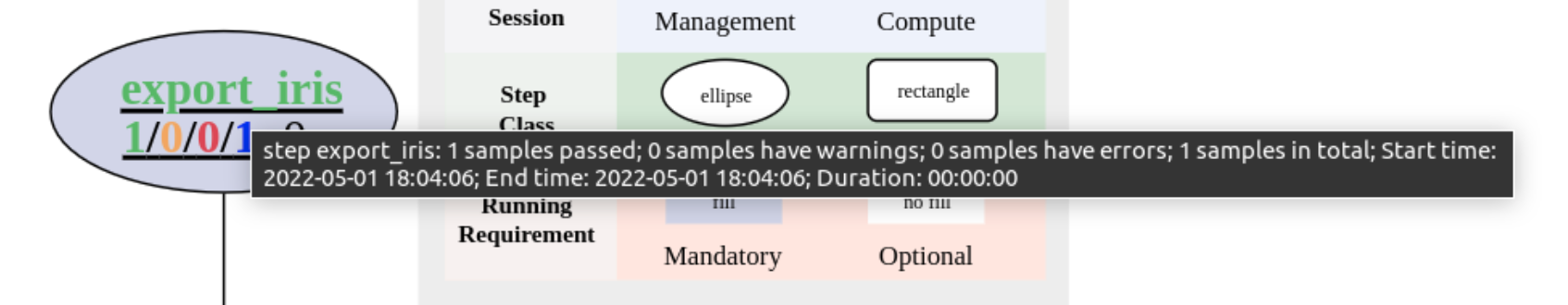
On hover
By default plotWF uses SVG to make the plot so it is interactive.
When the mouse is hovering on each step, detailed information will be displayed,
like sample information, processing time, duration, etc.
Embedding
In additional to SVG embedding, PNG embedding is supported, but the plot will no longer be interactively, good for browsers without optimal SVG support.
plotWF(sal, plot_method = "png", width = "80%")
Right click on the plot of SVG and PNG, we can see, SVGs are not directly savable, but PNGs are. However, PNGs are not vectorized, so it means it becomes blurry when we zoom in.
Responsiveness
This is a term often used in web development. It means will the plot resize itself if the user
resize the document window? By default, plotWF will be responsive, meaning it
will fit current window container size and adjust the size once the window size has
changed. To always display the full sized plot, use responsive = FALSE. It is useful
for embedding the plot in a full-screen mode.
plotWF(sal, responsive = FALSE, width = "80%")
Now resize your window width and watch plot above vs. other plots.
Pan-zoom
The Pan-zoom option enables users to drag the plot instead of scrolling, and to
use mouse wheel to zoom in/out. If you do not like the scroll bars in responsive = FALSE,
try this option. Note it cannot be used with responsive = TRUE together.
If both TRUE, responsive will be automatically set to FALSE. To enable this function
internet connection is required to download Javascript libraries on-the-fly.
plotWF(sal, pan_zoom = TRUE)
## Warning in plotWF(sal, pan_zoom = TRUE): Pan-zoom and responsive cannot be used
## together. Pan-zoom has priority, now `responsive` has set to FALSE
Layout
There a few different layout you can choose. There is no best layout. It all depends
on the workflow structure you have. The default is compact but we recommend you
to try different layouts to find the best fitting one.
compact: try to plot steps as close as possible.vertical: main branch will be placed vertically and side branches will be placed on the same horizontal level and sub steps of side branches will be placed vertically.horizontal: main branch is placed horizontally and side branches and sub steps will be placed vertically.execution: a linear plot to show the workflow execution order of all steps.
Here we are talking about the concept of main branch. It is a way to decide the plot center. We will discuss more below.
vertical
plotWF(sal, layout = "vertical", height = "600px")
If the plot is very long, use height to make it smaller.
horizontal
plotWF(sal, layout = "horizontal")
execution
plotWF(sal, layout = "execution", height = "600px", responsive = FALSE)
If the plot is too long, we can use height to limit it and/or use responsive
to make it scrollable.
Main branch
From the examples above, you can see that there are many steps which do not point to any other steps in downstream. These dead-ends are called ending steps. If we connect the first step, steps in between and these ending step, this will become a branch. Imagine the workflow is a top-bottom tree structure and the root is the first step. Therefore, there are many possible ways to connect the workflow. For the convenience of plotting, we introduce a concept of “main branch”, meaning one of the possible connecting strategies that will be placed at the center of the plot. Other steps that are not in this major branch will surround this major space. This “main branch” will not affect how a workflow is run, but just an algorithm to compute the best visualization. It will have impact on how we plot the workflow.
This main branch will not impact the compact layout so much but will have a huge
effect on horizontal and vertical layouts.
The algorithm in plotWF will automatically choose a best branch for
you by default. In simple words, it favors: (a). branches that connect first and last step;
(b). as long as possible.
You can also choose a branch you want by branch_method = "choose". It will first
list all possible branches, and then give you a prompt to ask for your favorite branch.
Here, for rendering the Rmarkdown, we cannot have a prompt, so we use a second argument
in combination, branch_no = x to directly choose a branch and skip the prompt. Also,
we use the verbose = TRUE to imitate the branch listing in console. In a real case,
you only need branch_method = "choose".
To have the main branch marked, mark_main_branch = TRUE must be added (default FALSE).
Watch closely how the plot change by choosing different branches. Here we use vertical
layout to demo. Remember, the main branch is marked in blue.
Choose branch 1
plotWF(sal, mark_main_branch = TRUE, layout = "vertical", branch_method = "choose", branch_no = 1, verbose = FALSE, height = "450px")
Choose branch 2
plotWF(sal, mark_main_branch = TRUE, layout = "vertical", branch_method = "choose", branch_no = 2, verbose = FALSE, height = "450px")
Do you see the difference?
Legends
The legend can also be removed by show_legend = FALSE
plotWF(sal, show_legend = FALSE, height = "500px")
Output formats
There are current three output formats: "html" and "dot", "dot_print". If first
two were chosen, you also need provide a path out_path to save the file.
- html: a single html file contains the plot.
- dot: a DOT script file with the code to reproduce the plot in a graphiz DOT engine.
- dot_print: directly cat the dot script to console.
HTML
HTML format is very useful if you want to view the plot later or share it to other
people. This format is also helpful when you are working on a remote computer
cluster. To view the workflow plot, a browser device (viewer) must be available,
but often time this is not the case for computer clusters. When you plot a workflow
and see the message "Couldn't get a file descriptor referring to the console",
it means your computer (cluster) does not have a browser device. Saving to
HTML format is the best option.
plotWF(sal, out_format = "html", out_path = "example_out.html")
file.exists("example_out.html")
## [1] TRUE
DOT
Saving workflow plot to dot format allows one to reproduce the plot with
the Graphviz language.
plotWF(sal, out_format = "dot", out_path = "example_out.dot")
file.exists("example_out.dot")
## [1] TRUE
DOT print
Instead of saving the Graphviz plotting code to a file, this option directly prints out the code on console. If you have a Graphviz plotting device in hand, simply copy and paste the code to that engine to reproduce the plot. For example, use our Workflow Plot Editor.
plotWF(sal, out_format = "dot_print")
Saving Static image file
Some users may want to save the plot to a static image, like .png format. We will
need do some extra work to save the file. The reason we cannot directly save it to
a png file is the plot is generated in real-time by a browser javascript engine. It
requires one type of javascript engine, like Chrome, MS Edge, Viewer in Rstudio,
to render the plot before we can see it, no matter you use SVG or PNG embedding.
Interactive
- With the
plot_ctr = TRUE(default) option, a plot control panel is displayed on the top-left corner. One can choose from different formats like png, jpg, svg or pdf to download them from the webpage. To enable these buttons, internet connection is required. The underlying Javascript libraries are download on-the-fly. Please make sure internet is connected. There are known conflicts of underlying web format creating libraries with R markdown web libraries, so some of these buttons may not work inside R markdown as you are seeing in this vignette right now. However, they should work properly if the workflow plot is saved to a stand-alone HTML file. - If you are working in Rstudio, you can also use the
exportbutton in the viewer to save an image file.
Note: due to the web libraries conflicts of this website and the libraries used in
plotWF. Some buttons may not work when you click, but it will work when you open make workflow plots interactively and view it in a stand-alone browser tab.
Non-interactive
If you cannot have an interactive session, like submitting a job to a cluster, but still want the png, we recommend to use the {webshot2} package to screenshot the plot. It runs headless Chrome in the back-end (which has a javascript engine).
Install the package
remotes::install_github("rstudio/webshot2")
Save to html first
plotWF(sal, out_format = "html", out_path = "example_out.html")
file.exists("example_out.html")
Use webshot2 to save the image
webshot2::webshot("example_out.html", "example_out.png")
In logs
The workflow steps will also become clickable if in_log = TRUE. This will create links
for each step that navigate to corresponding log section in the SPR
workflow log file. Normally this option
is handled by SPR log file generating function renderLogs to create this plot on top of the log file,
so when a certain step is click, it will navigate to the detailed section down the page.
Visit this page to see a real example. Try to click on the step in the workflow plot and watch what happens.
Session
sessionInfo()
## R version 4.2.0 (2022-04-22)
## Platform: x86_64-pc-linux-gnu (64-bit)
## Running under: Ubuntu 20.04.4 LTS
##
## Matrix products: default
## BLAS:   /usr/lib/x86_64-linux-gnu/blas/libblas.so.3.9.0
## LAPACK: /usr/lib/x86_64-linux-gnu/lapack/liblapack.so.3.9.0
##
## locale:
##  [1] LC_CTYPE=en_US.UTF-8       LC_NUMERIC=C
##  [3] LC_TIME=en_US.UTF-8        LC_COLLATE=en_US.UTF-8
##  [5] LC_MONETARY=en_US.UTF-8    LC_MESSAGES=en_US.UTF-8
##  [7] LC_PAPER=en_US.UTF-8       LC_NAME=C
##  [9] LC_ADDRESS=C               LC_TELEPHONE=C
## [11] LC_MEASUREMENT=en_US.UTF-8 LC_IDENTIFICATION=C
##
## attached base packages:
## [1] stats4    stats     graphics  grDevices utils     datasets  methods
## [8] base
##
## other attached packages:
##  [1] systemPipeR_2.3.4           ShortRead_1.54.0
##  [3] GenomicAlignments_1.32.0    SummarizedExperiment_1.26.1
##  [5] Biobase_2.56.0              MatrixGenerics_1.8.0
##  [7] matrixStats_0.62.0          BiocParallel_1.30.2
##  [9] Rsamtools_2.12.0            Biostrings_2.64.0
## [11] XVector_0.36.0              GenomicRanges_1.48.0
## [13] GenomeInfoDb_1.32.2         IRanges_2.30.0
## [15] S4Vectors_0.34.0            BiocGenerics_0.42.0
##
## loaded via a namespace (and not attached):
##  [1] lattice_0.20-45        png_0.1-7              assertthat_0.2.1
##  [4] digest_0.6.29          utf8_1.2.2             R6_2.5.1
##  [7] evaluate_0.15          highr_0.9              ggplot2_3.3.6
## [10] blogdown_1.10          pillar_1.7.0           zlibbioc_1.42.0
## [13] rlang_1.0.2            rstudioapi_0.13        jquerylib_0.1.4
## [16] Matrix_1.4-1           rmarkdown_2.14         labeling_0.4.2
## [19] stringr_1.4.0          htmlwidgets_1.5.4      RCurl_1.98-1.6
## [22] munsell_0.5.0          DelayedArray_0.22.0    compiler_4.2.0
## [25] xfun_0.31              pkgconfig_2.0.3        htmltools_0.5.2
## [28] tidyselect_1.1.2       tibble_3.1.7           GenomeInfoDbData_1.2.8
## [31] bookdown_0.26          fansi_1.0.3            dplyr_1.0.9
## [34] crayon_1.5.1           bitops_1.0-7           grid_4.2.0
## [37] DBI_1.1.2              jsonlite_1.8.0         gtable_0.3.0
## [40] lifecycle_1.0.1        magrittr_2.0.3         scales_1.2.0
## [43] cli_3.3.0              stringi_1.7.6          farver_2.1.0
## [46] hwriter_1.3.2.1        latticeExtra_0.6-29    bslib_0.3.1
## [49] generics_0.1.2         ellipsis_0.3.2         vctrs_0.4.1
## [52] RColorBrewer_1.1-3     tools_4.2.0            glue_1.6.2
## [55] purrr_0.3.4            jpeg_0.1-9             parallel_4.2.0
## [58] fastmap_1.1.0          yaml_2.3.5             colorspace_2.0-3
## [61] knitr_1.39             sass_0.4.1