SPatacseq
Author: Daniela Cassol (danielac@ucr.edu) and Thomas Girke (thomas.girke@ucr.edu)
Last update: 05 May, 2021
Source:vignettes/SPatacseq.Rmd
SPatacseq.RmdIntroduction
Users want to provide here background information about the design of their ATAC-Seq project.
ATAC-seq (Assay for Transposase-Accessible Chromatin with high-throughput sequencing) is a method to investigate the chromatin accessibility at a genome-wide level.
![ATAC-seq schematic methodology to chromatin accessibility using the Tn5 transposase.
In the open chromatin (line between nucleosomes in gray), Tn5 transposase (green) cuts the regions and insert the adaptors (red and blue) to generate sequencing-library
fragments. [@Buenrostro2013-ap]](Buenrostro2013.png)
ATAC-seq schematic methodology to chromatin accessibility using the Tn5 transposase. In the open chromatin (line between nucleosomes in gray), Tn5 transposase (green) cuts the regions and insert the adaptors (red and blue) to generate sequencing-library fragments. (Buenrostro et al. 2013)
SPatacseq pipeline will provide the steps to perform an ATAC-seq analysis. The pipeline show alternatives to trim adapters, check raw sequence read quality, alignment to the reference genome, call peaks, and visualization report.
Samples and environment settings
Required packages and resources
To go through this tutorial, you need the following software installed:
- R/>=4.0.3
- systemPipeR R package (version 1.24)
- bwa/0.7.17
The systemPipeR package (H Backman and Girke 2016) needs to be loaded to perform the analysis.
If you desire to build your pipeline with any different software, make sure to have the respective software installed and configured in your PATH. To make sure if the configuration is right, you always can test as follow:
tryCL(command = "bwa")
Structure of targets file
The targets file defines all input files (e.g. FASTQ, BAM, BCF) and sample comparisons of an analysis workflow. The following shows the format of a sample targets file included in the package. It also can be viewed and downloaded from systemPipeR’s GitHub repository here. In a target file with a single type of input files, here FASTQ files of single-end (SE) reads, the first three columns are mandatory including their column names, while it is four mandatory columns for FASTQ files of PE reads. All subsequent columns are optional and any number of additional columns can be added as needed.
Users should note here, the usage of targets files is optional when using systemPipeR’s new CWL interface. They can be replaced by a standard YAML input file used by CWL. Since for organizing experimental variables targets files are extremely useful and user-friendly. Thus, we encourage users to keep using them.
Structure of targets file for single-end (SE) samples
targetspath <- system.file("extdata", "targets.txt", package = "systemPipeR")
read.delim(targetspath, comment.char = "#")[1:4, ]
## FileName SampleName Factor SampleLong
## 1 ./data/SRR446027_1.fastq.gz M1A M1 Mock.1h.A
## 2 ./data/SRR446028_1.fastq.gz M1B M1 Mock.1h.B
## 3 ./data/SRR446029_1.fastq.gz A1A A1 Avr.1h.A
## 4 ./data/SRR446030_1.fastq.gz A1B A1 Avr.1h.B
## Experiment Date
## 1 1 23-Mar-2012
## 2 1 23-Mar-2012
## 3 1 23-Mar-2012
## 4 1 23-Mar-2012To work with custom data, users need to generate a targets file containing the paths to their own FASTQ files and then provide under targetspath the path to the corresponding targets file.
Quality control
Read Preprocessing
Preprocessing with preprocessReads function
The function preprocessReads allows to apply predefined or custom read preprocessing functions to all FASTQ files referenced in a SYSargs2 container, such as quality filtering or adaptor trimming routines. The paths to the resulting output FASTQ files are stored in the output slot of the SYSargs2 object. Internally, preprocessReads uses the FastqStreamer function from the ShortRead package to stream through large FASTQ files in a memory-efficient manner. The following example performs adaptor trimming with the trimLRPatterns function from the Biostrings package. After the trimming step a new targets file is generated (here targets_trimPE.txt) containing the paths to the trimmed FASTQ files. The new targets file can be used for the next workflow step with an updated SYSargs2 instance, e.g. running the NGS alignments with the trimmed FASTQ files.
Construct SYSargs2 object from cwl and yml param and targets files.
targetsPE <- system.file("extdata", "targetsPE.txt", package = "systemPipeR")
dir_path <- system.file("extdata/cwl/preprocessReads/trim-pe",
    package = "systemPipeR")
trim <- loadWorkflow(targets = targetsPE, wf_file = "trim-pe.cwl",
    input_file = "trim-pe.yml", dir_path = dir_path)
trim <- renderWF(trim, inputvars = c(FileName1 = "_FASTQ_PATH1_",
    FileName2 = "_FASTQ_PATH2_", SampleName = "_SampleName_"))
trim
output(trim)[1:2]
preprocessReads(args = trim, Fct = "trimLRPatterns(Rpattern='GCCCGGGTAA',
                subject=fq)",
    batchsize = 1e+05, overwrite = TRUE, compress = TRUE)
The following example shows how one can design a custom read preprocessing function using utilities provided by the ShortRead package, and then run it in batch mode with the ‘preprocessReads’ function (here on paired-end reads).
filterFct <- function(fq, cutoff = 20, Nexceptions = 0) {
    qcount <- rowSums(as(quality(fq), "matrix") <= cutoff, na.rm = TRUE)
    # Retains reads where Phred scores are >= cutoff with N
    # exceptions
    fq[qcount <= Nexceptions]
}
preprocessReads(args = trim, Fct = "filterFct(fq, cutoff=20, Nexceptions=0)",
    batchsize = 1e+05)
Preprocessing with TrimGalore!
TrimGalore! is a wrapper tool to consistently apply quality and adapter trimming to fastq files, with some extra functionality for removing Reduced Representation Bisulfite-Seq (RRBS) libraries.
targets <- system.file("extdata", "targets.txt", package = "systemPipeR")
dir_path <- system.file("extdata/cwl/trim_galore/trim_galore-se",
    package = "systemPipeR")
trimG <- loadWorkflow(targets = targets, wf_file = "trim_galore-se.cwl",
    input_file = "trim_galore-se.yml", dir_path = dir_path)
trimG <- renderWF(trimG, inputvars = c(FileName = "_FASTQ_PATH1_",
    SampleName = "_SampleName_"))
trimG
cmdlist(trimG)[1:2]
output(trimG)[1:2]
## Run Single Machine Option
trimG <- runCommandline(trimG[1], make_bam = FALSE)
Preprocessing with Trimmomatic
targetsPE <- system.file("extdata", "targetsPE.txt", package = "systemPipeR")
dir_path <- system.file("extdata/cwl/trimmomatic/trimmomatic-pe",
    package = "systemPipeR")
trimM <- loadWorkflow(targets = targetsPE, wf_file = "trimmomatic-pe.cwl",
    input_file = "trimmomatic-pe.yml", dir_path = dir_path)
trimM <- renderWF(trimM, inputvars = c(FileName1 = "_FASTQ_PATH1_",
    FileName2 = "_FASTQ_PATH2_", SampleName = "_SampleName_"))
trimM
cmdlist(trimM)[1:2]
output(trimM)[1:2]
## Run Single Machine Option
trimM <- runCommandline(trimM[1], make_bam = FALSE)
FASTQ quality report
The following seeFastq and seeFastqPlot functions generate and plot a series of useful quality statistics for a set of FASTQ files including per cycle quality box plots, base proportions, base-level quality trends, relative k-mer diversity, length and occurrence distribution of reads, number of reads above quality cutoffs and mean quality distribution.
The function seeFastq computes the quality statistics and stores the results in a relatively small list object that can be saved to disk with save() and reloaded with load() for later plotting. The argument klength specifies the k-mer length and batchsize the number of reads to a random sample from each FASTQ file.
fqlist <- seeFastq(fastq = infile1(trim), batchsize = 10000,
    klength = 8)
pdf("./results/fastqReport.pdf", height = 18, width = 4 * length(fqlist))
seeFastqPlot(fqlist)
dev.off()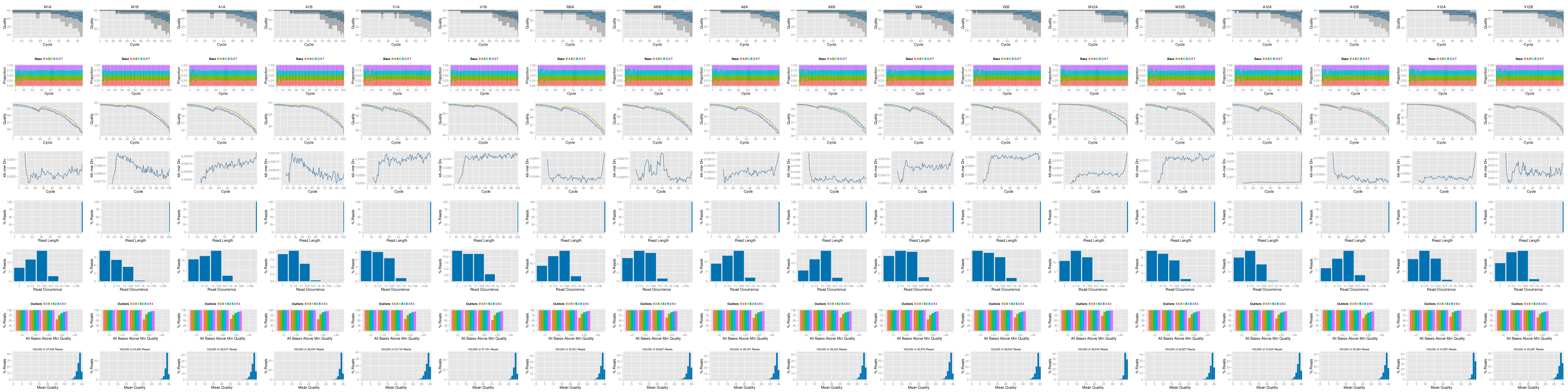
Parallelization of FASTQ quality report on a single machine with multiple cores.
f <- function(x) seeFastq(fastq = infile1(trim)[x], batchsize = 1e+05,
    klength = 8)
fqlist <- bplapply(seq(along = trim), f, BPPARAM = MulticoreParam(workers = 4))
seeFastqPlot(unlist(fqlist, recursive = FALSE))
Parallelization of FASTQ quality report via scheduler (e.g. Slurm) across several compute nodes.
library(BiocParallel)
library(batchtools)
f <- function(x) {
    library(systemPipeR)
    targetsPE <- system.file("extdata", "targetsPE.txt", package = "systemPipeR")
    dir_path <- system.file("extdata/cwl/preprocessReads/trim-pe",
        package = "systemPipeR")
    trim <- loadWorkflow(targets = targetsPE, wf_file = "trim-pe.cwl",
        input_file = "trim-pe.yml", dir_path = dir_path)
    trim <- renderWF(trim, inputvars = c(FileName1 = "_FASTQ_PATH1_",
        FileName2 = "_FASTQ_PATH2_", SampleName = "_SampleName_"))
    seeFastq(fastq = infile1(trim)[x], batchsize = 1e+05, klength = 8)
}
resources <- list(walltime = 120, ntasks = 1, ncpus = 4, memory = 1024)
param <- BatchtoolsParam(workers = 4, cluster = "slurm", template = "batchtools.slurm.tmpl",
    resources = resources)
fqlist <- bplapply(seq(along = trim), f, BPPARAM = param)
seeFastqPlot(unlist(fqlist, recursive = FALSE))
Read Alignment
After quality control, the sequence reads can be aligned to a reference genome or miRNA database. The following sessions present some NGS sequence alignment software. Select the most accurate aligner and determining the optimal parameter for your custom data set project.
For all the following examples, it is necessary to install the respective software and export the PATH accordingly. If it is available Environment Module in the system, you can load all the request software with moduleload(modules(idx)) function.
Alignment with Bowtie2
The following example runs Bowtie2 as a single process without submitting it to a cluster.
Building the index:
dir_path <- system.file("extdata/cwl/bowtie2/bowtie2-idx", package = "systemPipeR")
idx <- loadWorkflow(targets = NULL, wf_file = "bowtie2-index.cwl",
    input_file = "bowtie2-index.yml", dir_path = dir_path)
idx <- renderWF(idx)
idx
cmdlist(idx)

## Run in single machine
runCommandline(idx, make_bam = FALSE)
Building all the command-line:
targetspath <- system.file("extdata", "targetsPE.txt", package = "systemPipeR")
dir_path <- system.file("extdata/cwl/bowtie2/bowtie2-mi", package = "SPatacseq")
bowtie <- loadWorkflow(targets = targetspath, wf_file = "bowtie2-mapping-mi.cwl",
    input_file = "bowtie2-mapping-mi.yml", dir_path = dir_path)
bowtie <- renderWF(bowtie, inputvars = c(FileTrim = "_FASTQ_PATH1_",
    SampleName = "_SampleName_"))
bowtie
cmdlist(bowtie)[1:2]
output(bowtie)[1:2]
Please note that each experiment and/or each species may require an optimization of the parameters used. Here is an example where no mismatches are allowed, and -k mode is used. The -k represents the maximum number of alignments to report per read. By default, Bowtie2 reports at most one alignment per read, and if multiple equivalent alignments exist, it chooses one randomly. There is indicative that Bowtie2 with very sensitive local (--very-sensitive-local) argument provides better accuracy and generates smaller P-values for true positives (Ziemann, Kaspi, and El-Osta 2016).
Running all the jobs to computing nodes.
resources <- list(walltime = 120, ntasks = 1, ncpus = 4, memory = 1024)
reg <- clusterRun(bowtie, FUN = runCommandline, more.args = list(args = bowtiePE,
    dir = FALSE), conffile = ".batchtools.conf.R", template = "batchtools.slurm.tmpl",
    Njobs = 6, runid = "01", resourceList = resources)
getStatus(reg = reg)
bowtie <- output_update(bowtie, dir = FALSE, replace = TRUE,
    extension = c(".sam", ".bam"))
Alternatively, it possible to run all the jobs in a single machine.
bowtie <- runCommandline(bowtie, make_bam = TRUE)
systemPipeR:::check.output(bowtie)
Create new targets file.
names(clt(bowtie))
writeTargetsout(x = bowtie, file = "default", step = 1, new_col = "bowtie",
    new_col_output_index = 1, overwrite = TRUE)
Read and alignment count stats
Generate a table of read and alignment counts for all samples.
read_statsDF <- alignStats(bowtie, subset = "FileTrim")
write.table(read_statsDF, "results/alignStats_bowtie.xls", row.names = FALSE,
    quote = FALSE, sep = "\t")
The following shows the first four lines of the sample alignment stats file provided by the systemPipeR package.
table <- system.file("extdata", "alignStats.xls", package = "systemPipeR")
read.table(table, header = TRUE)
## FileName Nreads2x Nalign Perc_Aligned Nalign_Primary
## 1 M1A 192918 177961 92.24697 177961
## 2 M1B 197484 159378 80.70426 159378
## 3 A1A 189870 176055 92.72397 176055
## 4 A1B 188854 147768 78.24457 147768
## 5 V1A 198732 160115 80.56830 160115
## 6 V1B 195542 184418 94.31120 184418
## 7 M6A 197234 182469 92.51397 182469
## 8 M6B 180904 162636 89.90183 162636
## 9 A6A 183140 170258 92.96604 170258
## 10 A6B 196578 179932 91.53211 179932
## 11 V6A 194204 176857 91.06764 176857
## 12 V6B 198414 176825 89.11922 176825
## 13 M12A 199434 179722 90.11603 179722
## 14 M12B 188954 162894 86.20828 162894
## 15 A12A 187922 171326 91.16868 171326
## 16 A12B 199790 173771 86.97683 173771
## 17 V12A 193922 174180 89.81962 174180
## 18 V12B 181006 157790 87.17391 157790
## Perc_Aligned_Primary
## 1 92.24697
## 2 80.70426
## 3 92.72397
## 4 78.24457
## 5 80.56830
## 6 94.31120
## 7 92.51397
## 8 89.90183
## 9 92.96604
## 10 91.53211
## 11 91.06764
## 12 89.11922
## 13 90.11603
## 14 86.20828
## 15 91.16868
## 16 86.97683
## 17 89.81962
## 18 87.17391
Alignment with BWA-MEM (e.g. for VAR-Seq)
The following example runs BWA-MEM as a single process without submitting it to a cluster. ##TODO: add reference
Build the index:
dir_path <- system.file("extdata/cwl/bwa/bwa-idx", package = "systemPipeR")
idx <- loadWorkflow(targets = NULL, wf_file = "bwa-index.cwl",
    input_file = "bwa-index.yml", dir_path = dir_path)
idx <- renderWF(idx)
idx
cmdlist(idx)  # Indexes reference genome

## Run
runCommandline(idx, make_bam = FALSE)
Running the alignment:
targetsPE <- system.file("extdata", "targetsPE.txt", package = "systemPipeR")
dir_path <- system.file("extdata/cwl/bwa/bwa-pe", package = "systemPipeR")
bwaPE <- loadWorkflow(targets = targetsPE, wf_file = "bwa-pe.cwl",
    input_file = "bwa-pe.yml", dir_path = dir_path)
bwaPE <- renderWF(bwaPE, inputvars = c(FileName1 = "_FASTQ_PATH1_",
    FileName2 = "_FASTQ_PATH2_", SampleName = "_SampleName_"))
bwaPE
cmdlist(bwaPE)[1:2]
output(bwaPE)[1:2]
## Single Machine
bwaPE <- runCommandline(args = bwaPE, make_bam = TRUE)

## Cluster
library(batchtools)
resources <- list(walltime = 120, ntasks = 1, ncpus = 4, memory = 1024)
reg <- clusterRun(bwaPE, FUN = runCommandline, more.args = list(args = bwaPE,
    dir = FALSE), conffile = ".batchtools.conf.R", template = "batchtools.slurm.tmpl",
    Njobs = 18, runid = "01", resourceList = resources)
getStatus(reg = reg)
Create new targets file.
names(clt(bwaPE))
writeTargetsout(x = bwaPE, file = "default", step = 1, new_col = "bwaPE",
    new_col_output_index = 1, overwrite = TRUE)
Check whether all BAM files have been created and write out the new targets file.
writeTargetsout(x = bwaPE, file = "targets_bam.txt", step = 1,
    new_col = "FileName", new_col_output_index = 1, overwrite = TRUE)
outpaths <- subsetWF(args, slot = "output", subset = 1, index = 1)
file.exists(outpaths)
Create symbolic links for viewing BAM files in IGV
The symLink2bam function creates symbolic links to view the BAM alignment files in a genome browser such as IGV without moving these large files to a local system. The corresponding URLs are written to a file with a path specified under urlfile, here IGVurl.txt. Please replace the directory and the user name.
symLink2bam(sysargs = args, htmldir = c("~/.html/", "somedir/"),
    urlbase = "http://cluster.hpcc.ucr.edu/~tgirke/", urlfile = "./results/IGVurl.txt")
Utilities for coverage data
The following introduces several utilities useful for ChIP-Seq data. They are not part of the actual workflow.
Rle object stores coverage information
library(rtracklayer)
library(GenomicRanges)
library(Rsamtools)
library(GenomicAlignments)
outpaths <- subsetWF(bwaPE, slot = "output", subset = 1, index = 1)
aligns <- readGAlignments(outpaths[1])
cov <- coverage(aligns)
cov
# RleList of length 7 $Chr1 integer-Rle of length 100000 with
# 11827 runs Lengths: 3644 3 2 3 2 1 ...  1 5 23 3 12 Values
# : 0 1 3 4 5 6 ...  17 19 20 19 18 $Chr2 integer-Rle of
# length 100000 with 5085 runs Lengths: 999 7 11 55 2 5 ...
# 2 1 1 1 3357 Values : 0 2 3 4 3 2 ...  8 6 2 1 0 $Chr3
# integer-Rle of length 100000 with 12688 runs Lengths: 8953
# 5 1 2 9 5 ...  3 4 4 1 35 Values : 0 1 2 3 4 5 ...  16 15
# 14 2 0 $Chr4 integer-Rle of length 100000 with 5113 runs
# Lengths: 4104 53 157 71 4 50 ...  43 12 63 12 446 Values :
# 0 1 0 1 2 1 ...  0 1 2 1 0 $Chr5 integer-Rle of length
# 100000 with 6995 runs Lengths: 1236 34 1 2 1 1 ...  13 6 1
# 55 413 Values : 0 1 2 3 4 5 ...  5 4 3 1 0 ...  <2 more
# elements>Plot coverage for defined region
library(ggbio)
myloc <- c("Chr1", 1, 1e+05)
ga <- readGAlignments(outpaths[1], use.names = TRUE, param = ScanBamParam(which = GRanges(myloc[1],
    IRanges(as.numeric(myloc[2]), as.numeric(myloc[3])))))
autoplot(ga, aes(color = strand, fill = strand), facets = strand ~
    seqnames, stat = "coverage")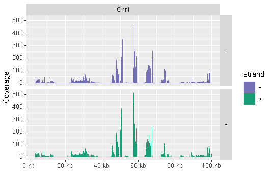
Peak calling with MACS2
Merge BAM files of replicates prior to peak calling
Merging BAM files of technical and/or biological replicates can improve the sensitivity of the peak calling by increasing the depth of read coverage. The mergeBamByFactor function merges BAM files based on grouping information specified by a factor, here the Factor column of the imported targets file. It also returns an updated SYSargs2 object containing the paths to the merged BAM files as well as to any unmerged files without replicates. This step can be skipped if merging of BAM files is not desired.
dir_path <- system.file("extdata/cwl/mergeBamByFactor", package = "systemPipeR")
args <- loadWF(targets = "targets_bam.txt", wf_file = "merge-bam.cwl",
    input_file = "merge-bam.yml", dir_path = dir_path)
args <- renderWF(args, inputvars = c(FileName = "_BAM_PATH_",
    SampleName = "_SampleName_"))

args_merge <- mergeBamByFactor(args = args, overwrite = TRUE)
writeTargetsout(x = args_merge, file = "targets_mergeBamByFactor.txt",
    step = 1, new_col = "FileName", new_col_output_index = 1,
overwrite = TRUE)Peak calling without input/reference sample
MACS2 can perform peak calling on ChIP-Seq data with and without input samples (Zhang et al. 2008). The following performs peak calling without input on all samples specified in the corresponding args object. Note, due to the small size of the sample data, MACS2 needs to be run here with the nomodel setting. For real data sets, users want to remove this parameter in the corresponding *.param file(s).
dir_path <- system.file("extdata/cwl/MACS2/MACS2-noinput/", package = "systemPipeR")
args <- loadWF(targets = "targets_mergeBamByFactor.txt", wf_file = "macs2.cwl",
    input_file = "macs2.yml", dir_path = dir_path)
args <- renderWF(args, inputvars = c(FileName = "_FASTQ_PATH1_",
    SampleName = "_SampleName_"))

runCommandline(args, make_bam = FALSE, force = T)
outpaths <- subsetWF(args, slot = "output", subset = 1, index = 1)
file.exists(outpaths)
writeTargetsout(x = args, file = "targets_macs.txt", step = 1,
    new_col = "FileName", new_col_output_index = 1, overwrite = TRUE)
Peak calling with input/reference sample
To perform peak calling with input samples, they can be most conveniently specified in the SampleReference column of the initial targets file. The writeTargetsRef function uses this information to create a targets file intermediate for running MACS2 with the corresponding input samples.
writeTargetsRef(infile = "targets_mergeBamByFactor.txt", outfile = "targets_bam_ref.txt",
    silent = FALSE, overwrite = TRUE)
dir_path <- system.file("extdata/cwl/MACS2/MACS2-input/", package = "systemPipeR")
args_input <- loadWF(targets = "targets_bam_ref.txt", wf_file = "macs2-input.cwl",
    input_file = "macs2.yml", dir_path = dir_path)
args_input <- renderWF(args_input, inputvars = c(FileName1 = "_FASTQ_PATH1_",
    FileName2 = "_FASTQ_PATH2_", SampleName = "_SampleName_"))
cmdlist(args_input)[1]
## Run
args_input <- runCommandline(args_input, make_bam = FALSE, force = T)
outpaths_input <- subsetWF(args_input, slot = "output", subset = 1,
    index = 1)
file.exists(outpaths_input)
writeTargetsout(x = args_input, file = "targets_macs_input.txt",
    step = 1, new_col = "FileName", new_col_output_index = 1,
    overwrite = TRUE)
The peak calling results from MACS2 are written for each sample to separate files in the results directory. They are named after the corresponding files with extensions used by MACS2.
Identify consensus peaks
The following example shows how one can identify consensus preaks among two peak sets sharing either a minimum absolute overlap and/or minimum relative overlap using the subsetByOverlaps or olRanges functions, respectively. Note, the latter is a custom function imported below by sourcing it.
# source('http://faculty.ucr.edu/~tgirke/Documents/R_BioCond/My_R_Scripts/rangeoverlapper.R')
outpaths <- subsetWF(args, slot = "output", subset = 1, index = 1)  ## escolher um dos outputs index
peak_M1A <- outpaths["M1A"]
peak_M1A <- as(read.delim(peak_M1A, comment = "#")[, 1:3], "GRanges")
peak_A1A <- outpaths["A1A"]
peak_A1A <- as(read.delim(peak_A1A, comment = "#")[, 1:3], "GRanges")
(myol1 <- subsetByOverlaps(peak_M1A, peak_A1A, minoverlap = 1))
# Returns any overlap
myol2 <- olRanges(query = peak_M1A, subject = peak_A1A, output = "gr")
# Returns any overlap with OL length information
myol2[values(myol2)["OLpercQ"][, 1] >= 50]
# Returns only query peaks with a minimum overlap of 50%
Annotate peaks with genomic context
Annotation with ChIPpeakAnno package
The following annotates the identified peaks with genomic context information using the ChIPpeakAnno and ChIPseeker packages, respectively (Zhu et al. 2010; Yu, Wang, and He 2015).
library(ChIPpeakAnno)
library(GenomicFeatures)
dir_path <- system.file("extdata/cwl/annotate_peaks", package = "systemPipeR")
args <- loadWF(targets = "targets_macs.txt", wf_file = "annotate-peaks.cwl",
    input_file = "annotate-peaks.yml", dir_path = dir_path)
args <- renderWF(args, inputvars = c(FileName = "_FASTQ_PATH1_",
    SampleName = "_SampleName_"))

txdb <- makeTxDbFromGFF(file = "data/tair10.gff", format = "gff",
    dataSource = "TAIR", organism = "Arabidopsis thaliana")
ge <- genes(txdb, columns = c("tx_name", "gene_id", "tx_type"))
for (i in seq(along = args)) {
    peaksGR <- as(read.delim(infile1(args)[i], comment = "#"),
        "GRanges")
    annotatedPeak <- annotatePeakInBatch(peaksGR, AnnotationData = genes(txdb))
    df <- data.frame(as.data.frame(annotatedPeak), as.data.frame(values(ge[values(annotatedPeak)$feature,
        ])))
    outpaths <- subsetWF(args, slot = "output", subset = 1, index = 1)
    write.table(df, outpaths[i], quote = FALSE, row.names = FALSE,
        sep = "\t")
}
writeTargetsout(x = args, file = "targets_peakanno.txt", step = 1,
    new_col = "FileName", new_col_output_index = 1, overwrite = TRUE)
The peak annotation results are written for each peak set to separate files in the results directory. They are named after the corresponding peak files with extensions specified in the annotate_peaks.param file, here *.peaks.annotated.xls.
Annotation with ChIPseeker package
Same as in previous step but using the ChIPseeker package for annotating the peaks.
library(ChIPseeker)
for (i in seq(along = args)) {
    peakAnno <- annotatePeak(infile1(args)[i], TxDb = txdb, verbose = FALSE)
    df <- as.data.frame(peakAnno)
    outpaths <- subsetWF(args, slot = "output", subset = 1, index = 1)
    write.table(df, outpaths[i], quote = FALSE, row.names = FALSE,
        sep = "\t")
}
writeTargetsout(x = args, file = "targets_peakanno.txt", step = 1,
    new_col = "FileName", new_col_output_index = 1, overwrite = TRUE)
Summary plots provided by the ChIPseeker package. Here applied only to one sample for demonstration purposes.
peak <- readPeakFile(infile1(args)[1])
covplot(peak, weightCol = "X.log10.pvalue.")
outpaths <- subsetWF(args, slot = "output", subset = 1, index = 1)
peakHeatmap(outpaths[1], TxDb = txdb, upstream = 1000, downstream = 1000,
    color = "red")
plotAvgProf2(outpaths[1], TxDb = txdb, upstream = 1000, downstream = 1000,
    xlab = "Genomic Region (5'->3')", ylab = "Read Count Frequency")
Count reads overlapping peaks
The countRangeset function is a convenience wrapper to perform read counting iteratively over serveral range sets, here peak range sets. Internally, the read counting is performed with the summarizeOverlaps function from the GenomicAlignments package. The resulting count tables are directly saved to files, one for each peak set.
library(GenomicRanges)
dir_path <- system.file("extdata/cwl/count_rangesets", package = "systemPipeR")
args <- loadWF(targets = "targets_macs.txt", wf_file = "count_rangesets.cwl",
    input_file = "count_rangesets.yml", dir_path = dir_path)
args <- renderWF(args, inputvars = c(FileName = "_FASTQ_PATH1_",
    SampleName = "_SampleName_"))

## Bam Files
targets <- system.file("extdata", "targetsPE_chip.txt", package = "systemPipeR")
dir_path <- system.file("extdata/cwl/bowtie2/bowtie2-pe", package = "systemPipeR")
args_bam <- loadWF(targets = targets, wf_file = "bowtie2-mapping-pe.cwl",
    input_file = "bowtie2-mapping-pe.yml", dir_path = dir_path)
args_bam <- renderWF(args_bam, inputvars = c(FileName = "_FASTQ_PATH1_",
    SampleName = "_SampleName_"))
args_bam <- output_update(args_bam, dir = FALSE, replace = TRUE,
    extension = c(".sam", ".bam"))
outpaths <- subsetWF(args_bam, slot = "output", subset = 1, index = 1)

bfl <- BamFileList(outpaths, yieldSize = 50000, index = character())
countDFnames <- countRangeset(bfl, args, mode = "Union", ignore.strand = TRUE)
writeTargetsout(x = args, file = "targets_countDF.txt", step = 1,
    new_col = "FileName", new_col_output_index = 1, overwrite = TRUE)
Differential binding analysis
The runDiff function performs differential binding analysis in batch mode for several count tables using edgeR or DESeq2 (Robinson, McCarthy, and Smyth 2010; Love, Huber, and Anders 2014). Internally, it calls the functions run_edgeR and run_DESeq2. It also returns the filtering results and plots from the downstream filterDEGs function using the fold change and FDR cutoffs provided under the dbrfilter argument.
dir_path <- system.file("extdata/cwl/rundiff", package = "systemPipeR")
args_diff <- loadWF(targets = "targets_countDF.txt", wf_file = "rundiff.cwl",
    input_file = "rundiff.yml", dir_path = dir_path)
args_diff <- renderWF(args_diff, inputvars = c(FileName = "_FASTQ_PATH1_",
    SampleName = "_SampleName_"))

cmp <- readComp(file = args_bam, format = "matrix")
dbrlist <- runDiff(args = args_diff, diffFct = run_edgeR, targets = targets.as.df(targets(args_bam)),
    cmp = cmp[[1]], independent = TRUE, dbrfilter = c(Fold = 2,
        FDR = 1))
writeTargetsout(x = args_diff, file = "targets_rundiff.txt",
    step = 1, new_col = "FileName", new_col_output_index = 1,
    overwrite = TRUE)
GO term enrichment analysis
The following performs GO term enrichment analysis for each annotated peak set.
dir_path <- system.file("extdata/cwl/annotate_peaks", package = "systemPipeR")
args <- loadWF(targets = "targets_bam_ref.txt", wf_file = "annotate-peaks.cwl",
    input_file = "annotate-peaks.yml", dir_path = dir_path)
args <- renderWF(args, inputvars = c(FileName1 = "_FASTQ_PATH1_",
    FileName2 = "_FASTQ_PATH2_", SampleName = "_SampleName_"))

args_anno <- loadWF(targets = "targets_macs.txt", wf_file = "annotate-peaks.cwl",
    input_file = "annotate-peaks.yml", dir_path = dir_path)
args_anno <- renderWF(args_anno, inputvars = c(FileName = "_FASTQ_PATH1_",
    SampleName = "_SampleName_"))
annofiles <- subsetWF(args_anno, slot = "output", subset = 1,
    index = 1)
gene_ids <- sapply(names(annofiles), function(x) unique(as.character(read.delim(annofiles[x])[,
    "geneId"])), simplify = FALSE)
load("data/GO/catdb.RData")
BatchResult <- GOCluster_Report(catdb = catdb, setlist = gene_ids,
    method = "all", id_type = "gene", CLSZ = 2, cutoff = 0.9,
    gocats = c("MF", "BP", "CC"), recordSpecGO = NULL)
Motif analysis
Parse DNA sequences of peak regions from genome
Enrichment analysis of known DNA binding motifs or de novo discovery of novel motifs requires the DNA sequences of the identified peak regions. To parse the corresponding sequences from the reference genome, the getSeq function from the Biostrings package can be used. The following example parses the sequences for each peak set and saves the results to separate FASTA files, one for each peak set. In addition, the sequences in the FASTA files are ranked (sorted) by increasing p-values as expected by some motif discovery tools, such as BCRANK.
library(Biostrings)
library(seqLogo)
library(BCRANK)
dir_path <- system.file("extdata/cwl/annotate_peaks", package = "systemPipeR")
args <- loadWF(targets = "targets_macs.txt", wf_file = "annotate-peaks.cwl",
    input_file = "annotate-peaks.yml", dir_path = dir_path)
args <- renderWF(args, inputvars = c(FileName = "_FASTQ_PATH1_",
    SampleName = "_SampleName_"))

rangefiles <- infile1(args)
for (i in seq(along = rangefiles)) {
    df <- read.delim(rangefiles[i], comment = "#")
    peaks <- as(df, "GRanges")
    names(peaks) <- paste0(as.character(seqnames(peaks)), "_",
        start(peaks), "-", end(peaks))
    peaks <- peaks[order(values(peaks)$X.log10.pvalue., decreasing = TRUE)]
    pseq <- getSeq(FaFile("./data/tair10.fasta"), peaks)
    names(pseq) <- names(peaks)
    writeXStringSet(pseq, paste0(rangefiles[i], ".fasta"))
}
Motif discovery with BCRANK
The Bioconductor package BCRANK is one of the many tools available for de novo discovery of DNA binding motifs in peak regions of ChIP-Seq experiments. The given example applies this method on the first peak sample set and plots the sequence logo of the highest ranking motif.
set.seed(0)
BCRANKout <- bcrank(paste0(rangefiles[1], ".fasta"), restarts = 25,
    use.P1 = TRUE, use.P2 = TRUE)
toptable(BCRANKout)
topMotif <- toptable(BCRANKout, 1)
weightMatrix <- pwm(topMotif, normalize = FALSE)
weightMatrixNormalized <- pwm(topMotif, normalize = TRUE)
pdf("results/seqlogo.pdf")
seqLogo(weightMatrixNormalized)
dev.off()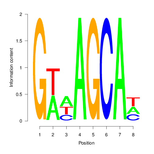
BCRANK
Version Information
## R Under development (unstable) (2021-02-04 r79940)
## Platform: x86_64-pc-linux-gnu (64-bit)
## Running under: Ubuntu 20.04.2 LTS
##
## Matrix products: default
## BLAS:   /usr/lib/x86_64-linux-gnu/blas/libblas.so.3.9.0
## LAPACK: /home/dcassol/src/R-devel/lib/libRlapack.so
##
## locale:
##  [1] LC_CTYPE=en_US.UTF-8       LC_NUMERIC=C
##  [3] LC_TIME=en_US.UTF-8        LC_COLLATE=en_US.UTF-8
##  [5] LC_MONETARY=en_US.UTF-8    LC_MESSAGES=en_US.UTF-8
##  [7] LC_PAPER=en_US.UTF-8       LC_NAME=C
##  [9] LC_ADDRESS=C               LC_TELEPHONE=C
## [11] LC_MEASUREMENT=en_US.UTF-8 LC_IDENTIFICATION=C
##
## attached base packages:
## [1] stats4    parallel  stats     graphics  grDevices
## [6] utils     datasets  methods   base
##
## other attached packages:
##  [1] systemPipeR_1.25.11         ShortRead_1.49.2
##  [3] GenomicAlignments_1.27.2    SummarizedExperiment_1.21.3
##  [5] Biobase_2.51.0              MatrixGenerics_1.3.1
##  [7] matrixStats_0.58.0          BiocParallel_1.25.5
##  [9] Rsamtools_2.7.2             Biostrings_2.59.2
## [11] XVector_0.31.1              GenomicRanges_1.43.4
## [13] GenomeInfoDb_1.27.11        IRanges_2.25.9
## [15] S4Vectors_0.29.15           BiocGenerics_0.37.2
## [17] BiocStyle_2.19.2
##
## loaded via a namespace (and not attached):
##   [1] colorspace_2.0-0         rjson_0.2.20
##   [3] hwriter_1.3.2            ellipsis_0.3.1
##   [5] rprojroot_2.0.2          fs_1.5.0
##   [7] bit64_4.0.5              AnnotationDbi_1.53.1
##   [9] fansi_0.4.2              codetools_0.2-18
##  [11] cachem_1.0.4             knitr_1.32
##  [13] jsonlite_1.7.2           annotate_1.69.2
##  [15] dbplyr_2.1.1             png_0.1-7
##  [17] BiocManager_1.30.12      compiler_4.1.0
##  [19] httr_1.4.2               backports_1.2.1
##  [21] assertthat_0.2.1         Matrix_1.3-2
##  [23] fastmap_1.1.0            limma_3.47.12
##  [25] formatR_1.9              htmltools_0.5.1.1
##  [27] prettyunits_1.1.1        tools_4.1.0
##  [29] gtable_0.3.0             glue_1.4.2
##  [31] GenomeInfoDbData_1.2.4   dplyr_1.0.5
##  [33] rsvg_2.1.1               batchtools_0.9.15
##  [35] rappdirs_0.3.3           V8_3.4.0
##  [37] Rcpp_1.0.6               jquerylib_0.1.3
##  [39] pkgdown_1.6.1            vctrs_0.3.7
##  [41] rtracklayer_1.51.5       xfun_0.22
##  [43] stringr_1.4.0            lifecycle_1.0.0
##  [45] restfulr_0.0.13          XML_3.99-0.6
##  [47] edgeR_3.33.3             scales_1.1.1
##  [49] zlibbioc_1.37.0          BSgenome_1.59.2
##  [51] VariantAnnotation_1.37.1 ragg_1.1.2
##  [53] hms_1.0.0                RColorBrewer_1.1-2
##  [55] yaml_2.2.1               curl_4.3
##  [57] memoise_2.0.0            ggplot2_3.3.3
##  [59] sass_0.3.1               biomaRt_2.47.7
##  [61] latticeExtra_0.6-29      stringi_1.5.3
##  [63] RSQLite_2.2.7            highr_0.9
##  [65] BiocIO_1.1.2             desc_1.3.0
##  [67] checkmate_2.0.0          GenomicFeatures_1.43.8
##  [69] filelock_1.0.2           DOT_0.1
##  [71] rlang_0.4.10             pkgconfig_2.0.3
##  [73] systemfonts_1.0.1        bitops_1.0-6
##  [75] evaluate_0.14            lattice_0.20-41
##  [77] purrr_0.3.4              bit_4.0.4
##  [79] tidyselect_1.1.0         magrittr_2.0.1
##  [81] bookdown_0.22            R6_2.5.0
##  [83] generics_0.1.0           base64url_1.4
##  [85] DelayedArray_0.17.10     DBI_1.1.1
##  [87] pillar_1.6.0             withr_2.4.2
##  [89] KEGGREST_1.31.1          RCurl_1.98-1.3
##  [91] tibble_3.1.1             crayon_1.4.1
##  [93] utf8_1.2.1               BiocFileCache_1.99.6
##  [95] rmarkdown_2.7            jpeg_0.1-8.1
##  [97] progress_1.2.2           locfit_1.5-9.4
##  [99] grid_4.1.0               data.table_1.14.0
## [101] blob_1.2.1               digest_0.6.27
## [103] xtable_1.8-4             brew_1.0-6
## [105] textshaping_0.3.3        munsell_0.5.0
## [107] bslib_0.2.4
Funding
This project was supported by funds from the National Institutes of Health (NIH) and the National Science Foundation (NSF).