systemPipeShiny

class: center, middle, inverse, title-slide

# <img src="https://raw.githubusercontent.com/systemPipeR/systemPipeShiny/master/inst/app/www/img/sps_small.png" style="width:1in" /> systemPipeShiny
### Daniela Cassol & Le Zhang
### <h3>
University of California Riverside
<h3/>
### <h3>
2020/08/28 (updated: 2020-08-31)
<h3/>

---

layout: true
background-image: url(https://raw.githubusercontent.com/systemPipeR/systemPipeShiny/master/inst/app/www/img/sps_small.png)
background-position: 100% 0%
background-size: 10%

---
class: center, middle

## Outline

#### Introduction
#### *systemPipeShiny* Demo
#### Visualization Features
#### Customize and Extend
---
class: inverse, center, middle

# Introduction

---
## Motivation

Build an interactive framework for workflow management and visualization by extending all [systemPipeR](https://systempipe.org/) functionalities

.pull-left[
![](overview1.png)
]
.pull-right[
![](targets.png)
]

---
## Motivation

.pull-left[
![](overview1.png)
]
.pull-right[

![](test.png)
]

---
## Motivation

.pull-left[
.center[
![](overview2.png)
]]
.pull-right[

<a href="#add link"><img src="qual.png" width="190" height="440" title=targets alt=Targets></a>
]

---
## Motivation

.pull-left[
![](overview3.png)
]
.pull-right[

<a href="#heatMap"><img src="heat_samples.svg"width="150" height="150" title=#heatMap alt=heat_samples.svg></a><a href="#cor"><img src="cor.svg"width="150" height="150" title=#cor alt=cor.svg></a><a href="#pca"><img src="tsne.svg"width="150" height="150" title=#pca alt=tsne.svg></a><a href="#volcano"><img src="volcano.svg"width="150" height="150" title=#volcano alt=volcano.svg></a><a href="#volcano"><img src="heat.png"width="150" height="150" title=#volcano alt=heat.png></a><a href="#logs"><img src="maplot.svg"width="150" height="150" title=#logs alt=maplot.svg></a>
]

---
## Motivation

.pull-left[
![](overview4.png)
]
.pull-right[
![](canvas.png)
]

---

## Motivation

Provide for non-R users, such as experimentalists, to run many systemPipeR’s workflow designs, control, and visualization functionalities interactively without requiring knowledge of R

Provide a tool that can be used on both local computers as well as centralized server-based deployments that can be accessed remotely as a public web service for using SPR’s functionalities with the community and/or private data

---
## Features

.middle-slide[
![](images/systemPipeShiny.png)
]

???

Interactively define experimental designs and provide associated metadata
using an easy to use tabular editor and/or file uploader

visualize workflow topologies combined with auto-generation of R Markdown previews for
interactively designed workflows

Allows prepare the data for the visualizations tabs

---
## Structural Features

.left-column[
### User friendly
]

.right-column[
![](sps_plot.png) 
]

---

## Structural Features

.left-column[
### User friendly
### Progress Tracking
]

.right-column[

![](sps_plot.png)

]

---
## Structural Features

.left-column[
### User friendly
### Progress Tracking
### Canvas 
]

.right-column[
Under this workbench users can take snapshots of different plots, and combine or resize them. This
feature is useful for generating complex scientific summary graphics.

<img src="canvas.png" alt="drawing" style="width:450px;"/>
]

---
## Structural Features

.left-column[
### Progress Tracking
]

.right-column[
Messages, warnings and errors from R functions are automatically captured and logged on
both the server and client ends.

<img src="error.png" alt="drawing" style="width:450px;"/>
]

---
## Structural Features

.left-column[
### Progress Tracking
### App Config
]

.right-column[
a robust exception handling system has been implemented (similar to Shiny options), that
provides error solutions to to users, e.g. invalid parameter settings.
]

---
## Structural Features

.left-column[
### Progress Tracking
### App Config
### Modular Design
]

.right-column[
SPS is built on Shiny modules, which provides local scope isolation between each tab.
Objects on one tab do not conflict with other tabs. To enable cross-tab communication, SPS also supports
global scope interactions
]

---
## Design

![](systemPipeShiny.png)
---
## Customize and Extend

Templates are available to generate new visualization tabs

![](images/sps_custom.png)

---
class: inverse, center, middle

# Live Demo

---
## Install Package

Install the **systemPipeShiny** package from [GitHub](https://github.com/systemPipeR/systemPipeShiny):

```r
if (!requireNamespace("BiocManager", quietly=TRUE))
    install.packages("BiocManager")
BiocManager::install("systemPipeR/systemPipeShiny", dependencies=TRUE, build_vignettes=TRUE)
```

### Load Package and Documentation

Load packages and accessing help

```r
library("systemPipeShiny")
```

Access help

```r
library(help="systemPipeShiny")
vignette("systemPipeShiny")
```

---
## Quick Start

Create the project:

```r
systemPipeShiny::spsInit()

## [SPS-INFO] 2020-08-30 17:03:28 Start to create a new SPS project
## [SPS-INFO] 2020-08-30 17:03:28 Create project under /home/dcassol/danielac@ucr.edu/projects/Presentations/SPS/SPS_20200830
## [SPS-INFO] 2020-08-30 17:03:28 Now copy files
## [SPS-INFO] 2020-08-30 17:03:28 Create SPS database
## [SPS-INFO] 2020-08-30 17:03:28 Created SPS database method container
## [SPS-INFO] 2020-08-30 17:03:28 Creating SPS db...
## [SPS-DANGER] 2020-08-30 17:03:28 Db created at '/home/dcassol/danielac@ucr.edu/projects/Presentations/SPS/SPS_20200830/config/sps.db'. DO NOT share this file with others
## [SPS-INFO] 2020-08-30 17:03:28 Key md5 dc17b12b7cadbb70e2d32a77bb32a17f
## [SPS-INFO] 2020-08-30 17:03:28 SPS project setup done!
```

---
## SPS Folder Structure

Directory structure:

```
SPS_YYYYMMDD
├── server.R
├── ui.R
├── global.R ## It will need manual input for new tabs
├── deploy.R ## Deploy helper file
├── config/ ## Folder with app configuration files
│   ├── sps.db             
│   ├── sps_options.yaml   
│   └── tabs.csv  
├── R/ ## All SPS additional tab files and helper R function files
│   └── tabs_xx.R 
├── data/ ## Storage all the input data
│   └── inputData 
├── results/ ## Storage all the results and plot data
│   └── plot_xx.png 
└── www/ ## Folder with all the app resources
```

---
## Launching the interface

The `runApp` function from `shiny` package launches the app in our browser.

```r
shiny::runApp()
```

Check out our instance of **systemPipeShiny**: [Link](https://tgirke.shinyapps.io/systemPipeShiny/)

Note: Add iframe here

---
class: inverse, center, middle

# Visualization Features

---

### Data transformations and visualization

.panelset[
.panel[.panel-name[Plot]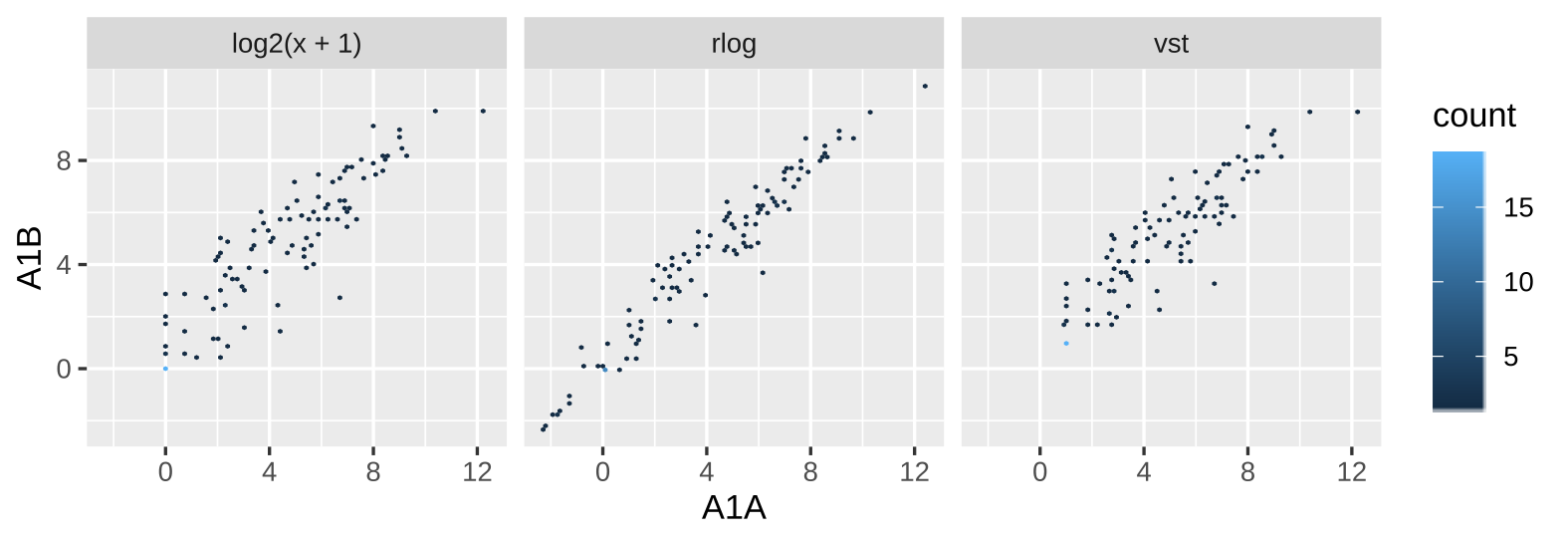
![](transf2.png)
]

.panel[
.panel-name[
R Code
]

```r
targetspath <- system.file("extdata", "targets.txt", package = "systemPipeR")
targets <- read.delim(targetspath, comment = "#")
cmp <- systemPipeR::readComp(file = targetspath, format = "matrix", delim = "-")
countMatrixPath <- system.file("extdata", "countDFeByg.xls", package = "systemPipeR")
countMatrix <- read.delim(countMatrixPath, row.names = 1)
exploreDDSplot(countMatrix, targets, cmp = cmp[[1]], preFilter = NULL,
 samples = c(3, 4), savePlot = TRUE, filePlot = "transf.png")
```
]
]

---

### Heatmap

.panelset[
.panel[.panel-name[Samples]
<img src="heat_samples.svg" height="425px" class="center" />
]

.panel[.panel-name[Individuals]
<img src="heat_ind.svg" height="425px" class="center" />
]

.panel[
.panel-name[R Code]
#### Samples

```r
exploredds <- exploreDDS(countMatrix, targets, cmp=cmp[[1]], preFilter=NULL, transformationMethod="rlog")
heatMaplot(exploredds, clust="samples")
heatMaplot(exploredds, clust="samples", plotly = TRUE)
```

#### Individuals genes identified in DEG analysis

```r
### DEG analysis with `systemPipeR`
degseqDF <- systemPipeR::run_DESeq2(countDF = countMatrix, targets = targets, cmp = cmp[[1]], independent = FALSE)
DEG_list <- systemPipeR::filterDEGs(degDF = degseqDF, filter = c(Fold = 2, FDR = 10))
heatMaplot(exploredds, clust="ind", DEGlist = unique(as.character(unlist(DEG_list[[1]]))))
heatMaplot(exploredds, clust="ind", DEGlist = unique(as.character(unlist(DEG_list[[1]]))), plotly = TRUE)
```

]]

---

### Dendrogram

.panelset[
.panel[.panel-name[Plot]
<img src="cor.svg" height="425px" class="center" />
]

.panel[
.panel-name[
R Code
]

```r
exploredds <- exploreDDS(countMatrix, targets, cmp=cmp[[1]], preFilter=NULL, transformationMethod="rlog")
hclustplot(exploredds, method = "spearman")
hclustplot(exploredds, method = "spearman", savePlot = TRUE, filePlot = "cor.pdf")
```
]
]

---

### PCA plot

.panelset[
.panel[.panel-name[Plot plotly]
<div id="htmlwidget-56a5ba518973d0773b79" style="width:504px;height:504px;" class="plotly html-widget"></div>
<script type="application/json" data-for="htmlwidget-56a5ba518973d0773b79">{"x":{"data":[{"x":[-3.03168381476885,-6.03412691707515],"y":[-0.535073099413187,-2.0971750907225],"text":["colour: A1 PC1: -3.0316838 PC2: -0.5350731","colour: A1 PC1: -6.0341269 PC2: -2.0971751"],"type":"scatter","mode":"markers","marker":{"autocolorscale":false,"color":"rgba(248,118,109,1)","opacity":1,"size":11.3385826771654,"symbol":"circle","line":{"width":1.88976377952756,"color":"rgba(248,118,109,1)"}},"hoveron":"points","name":"A1","legendgroup":"A1","showlegend":true,"xaxis":"x","yaxis":"y","hoverinfo":"text","frame":null},{"x":[3.88869312311426,-0.383756141678079],"y":[0.0701335027868824,4.53821439195817],"text":["colour: A12 PC1: 3.8886931 PC2: 0.0701335","colour: A12 PC1: -0.3837561 PC2: 4.5382144"],"type":"scatter","mode":"markers","marker":{"autocolorscale":false,"color":"rgba(211,146,0,1)","opacity":1,"size":11.3385826771654,"symbol":"circle","line":{"width":1.88976377952756,"color":"rgba(211,146,0,1)"}},"hoveron":"points","name":"A12","legendgroup":"A12","showlegend":true,"xaxis":"x","yaxis":"y","hoverinfo":"text","frame":null},{"x":[3.28184331604165,-0.416809087724184],"y":[0.185372641000547,5.30010399483779],"text":["colour: A6 PC1: 3.2818433 PC2: 0.1853726","colour: A6 PC1: -0.4168091 PC2: 5.3001040"],"type":"scatter","mode":"markers","marker":{"autocolorscale":false,"color":"rgba(147,170,0,1)","opacity":1,"size":11.3385826771654,"symbol":"circle","line":{"width":1.88976377952756,"color":"rgba(147,170,0,1)"}},"hoveron":"points","name":"A6","legendgroup":"A6","showlegend":true,"xaxis":"x","yaxis":"y","hoverinfo":"text","frame":null},{"x":[-4.23478929449673,-5.72288504075975],"y":[2.46441944072604,-1.3362445127839],"text":["colour: M1 PC1: -4.2347893 PC2: 2.4644194","colour: M1 PC1: -5.7228850 PC2: -1.3362445"],"type":"scatter","mode":"markers","marker":{"autocolorscale":false,"color":"rgba(0,186,56,1)","opacity":1,"size":11.3385826771654,"symbol":"circle","line":{"width":1.88976377952756,"color":"rgba(0,186,56,1)"}},"hoveron":"points","name":"M1","legendgroup":"M1","showlegend":true,"xaxis":"x","yaxis":"y","hoverinfo":"text","frame":null},{"x":[3.08219911545694,4.0916538760623],"y":[-1.26931397709069,-3.52388688937858],"text":["colour: M12 PC1: 3.0821991 PC2: -1.2693140","colour: M12 PC1: 4.0916539 PC2: -3.5238869"],"type":"scatter","mode":"markers","marker":{"autocolorscale":false,"color":"rgba(0,193,159,1)","opacity":1,"size":11.3385826771654,"symbol":"circle","line":{"width":1.88976377952756,"color":"rgba(0,193,159,1)"}},"hoveron":"points","name":"M12","legendgroup":"M12","showlegend":true,"xaxis":"x","yaxis":"y","hoverinfo":"text","frame":null},{"x":[2.40175386965523,1.53523865252027],"y":[1.67449958551854,0.392038639964049],"text":["colour: M6 PC1: 2.4017539 PC2: 1.6744996","colour: M6 PC1: 1.5352387 PC2: 0.3920386"],"type":"scatter","mode":"markers","marker":{"autocolorscale":false,"color":"rgba(0,185,227,1)","opacity":1,"size":11.3385826771654,"symbol":"circle","line":{"width":1.88976377952756,"color":"rgba(0,185,227,1)"}},"hoveron":"points","name":"M6","legendgroup":"M6","showlegend":true,"xaxis":"x","yaxis":"y","hoverinfo":"text","frame":null},{"x":[-4.10114199086997,-5.13397514161901],"y":[-0.524772724724376,-2.59419479868824],"text":["colour: V1 PC1: -4.1011420 PC2: -0.5247727","colour: V1 PC1: -5.1339751 PC2: -2.5941948"],"type":"scatter","mode":"markers","marker":{"autocolorscale":false,"color":"rgba(97,156,255,1)","opacity":1,"size":11.3385826771654,"symbol":"circle","line":{"width":1.88976377952756,"color":"rgba(97,156,255,1)"}},"hoveron":"points","name":"V1","legendgroup":"V1","showlegend":true,"xaxis":"x","yaxis":"y","hoverinfo":"text","frame":null},{"x":[2.70779870992001,1.85669227563915],"y":[-0.325101355885941,1.77346995606566],"text":["colour: V12 PC1: 2.7077987 PC2: -0.3251014","colour: V12 PC1: 1.8566923 PC2: 1.7734700"],"type":"scatter","mode":"markers","marker":{"autocolorscale":false,"color":"rgba(219,114,251,1)","opacity":1,"size":11.3385826771654,"symbol":"circle","line":{"width":1.88976377952756,"color":"rgba(219,114,251,1)"}},"hoveron":"points","name":"V12","legendgroup":"V12","showlegend":true,"xaxis":"x","yaxis":"y","hoverinfo":"text","frame":null},{"x":[3.29098889669914,2.92230559388278],"y":[-0.928463576912153,-3.26402612725811],"text":["colour: V6 PC1: 3.2909889 PC2: -0.9284636","colour: V6 PC1: 2.9223056 PC2: -3.2640261"],"type":"scatter","mode":"markers","marker":{"autocolorscale":false,"color":"rgba(255,97,195,1)","opacity":1,"size":11.3385826771654,"symbol":"circle","line":{"width":1.88976377952756,"color":"rgba(255,97,195,1)"}},"hoveron":"points","name":"V6","legendgroup":"V6","showlegend":true,"xaxis":"x","yaxis":"y","hoverinfo":"text","frame":null}],"layout":{"margin":{"t":40.8401826484018,"r":7.30593607305936,"b":37.2602739726027,"l":37.2602739726027},"plot_bgcolor":"rgba(235,235,235,1)","paper_bgcolor":"rgba(255,255,255,1)","font":{"color":"rgba(0,0,0,1)","family":"","size":14.6118721461187},"title":{"text":"Principal Component Analysis (PCA)","font":{"color":"rgba(0,0,0,1)","family":"","size":17.5342465753425},"x":0,"xref":"paper"},"xaxis":{"domain":[0,1],"automargin":true,"type":"linear","autorange":false,"range":[-6.54041595673202,4.59794291571917],"tickmode":"array","ticktext":["-6","-4","-2","0","2","4"],"tickvals":[-6,-4,-2,0,2,4],"categoryorder":"array","categoryarray":["-6","-4","-2","0","2","4"],"nticks":null,"ticks":"outside","tickcolor":"rgba(51,51,51,1)","ticklen":3.65296803652968,"tickwidth":0.66417600664176,"showticklabels":true,"tickfont":{"color":"rgba(77,77,77,1)","family":"","size":11.689497716895},"tickangle":-0,"showline":false,"linecolor":null,"linewidth":0,"showgrid":true,"gridcolor":"rgba(255,255,255,1)","gridwidth":0.66417600664176,"zeroline":false,"anchor":"y","title":{"text":"PC1: 39% variance","font":{"color":"rgba(0,0,0,1)","family":"","size":14.6118721461187}},"scaleanchor":"y","scaleratio":1,"hoverformat":".2f"},"yaxis":{"domain":[0,1],"automargin":true,"type":"linear","autorange":false,"range":[-3.9650864335894,5.74130353904861],"tickmode":"array","ticktext":["-2","0","2","4"],"tickvals":[-2,0,2,4],"categoryorder":"array","categoryarray":["-2","0","2","4"],"nticks":null,"ticks":"outside","tickcolor":"rgba(51,51,51,1)","ticklen":3.65296803652968,"tickwidth":0.66417600664176,"showticklabels":true,"tickfont":{"color":"rgba(77,77,77,1)","family":"","size":11.689497716895},"tickangle":-0,"showline":false,"linecolor":null,"linewidth":0,"showgrid":true,"gridcolor":"rgba(255,255,255,1)","gridwidth":0.66417600664176,"zeroline":false,"anchor":"x","title":{"text":"PC2: 17% variance","font":{"color":"rgba(0,0,0,1)","family":"","size":14.6118721461187}},"scaleanchor":"x","scaleratio":1,"hoverformat":".2f"},"shapes":[{"type":"rect","fillcolor":null,"line":{"color":null,"width":0,"linetype":[]},"yref":"paper","xref":"paper","x0":0,"x1":1,"y0":0,"y1":1}],"showlegend":true,"legend":{"bgcolor":"rgba(255,255,255,1)","bordercolor":"transparent","borderwidth":1.88976377952756,"font":{"color":"rgba(0,0,0,1)","family":"","size":11.689497716895},"y":0.938132733408324},"annotations":[{"text":"colour","x":1.02,"y":1,"showarrow":false,"ax":0,"ay":0,"font":{"color":"rgba(0,0,0,1)","family":"","size":14.6118721461187},"xref":"paper","yref":"paper","textangle":-0,"xanchor":"left","yanchor":"bottom","legendTitle":true}],"hovermode":"closest","barmode":"relative"},"config":{"doubleClick":"reset","showSendToCloud":false},"source":"A","attrs":{"3a05f57e01ae":{"colour":{},"x":{},"y":{},"type":"scatter"}},"cur_data":"3a05f57e01ae","visdat":{"3a05f57e01ae":["function (y) ","x"]},"highlight":{"on":"plotly_click","persistent":false,"dynamic":false,"selectize":false,"opacityDim":0.2,"selected":{"opacity":1},"debounce":0},"shinyEvents":["plotly_hover","plotly_click","plotly_selected","plotly_relayout","plotly_brushed","plotly_brushing","plotly_clickannotation","plotly_doubleclick","plotly_deselect","plotly_afterplot","plotly_sunburstclick"],"base_url":"https://plot.ly"},"evals":[],"jsHooks":[]}</script>
]

.panel[.panel-name[Plot ggplot2]
<img src="pca.svg" height="425px" class="center" />
]

.panel[
.panel-name[
R Code
]

```r
library(systemPipeShiny)
targetspath <- system.file("extdata", "targets.txt", package="systemPipeR")
targets <- read.delim(targetspath, comment="#")
cmp <- systemPipeR::readComp(file=targetspath, format="matrix", delim="-")
countMatrixPath <- system.file("extdata", "countDFeByg.xls", package="systemPipeR")
countMatrix <- read.delim(countMatrixPath, row.names=1)
exploredds <- exploreDDS(countMatrix, targets, cmp=cmp[[1]], preFilter=NULL, transformationMethod="rlog")
PCAplot(exploredds, plotly = TRUE)
```
]
]

---

### Multidimensional Scaling (MDS) plot

.panelset[
.panel[.panel-name[Plot]
<img src="mds.svg" height="425px" class="center" />
]

.panel[
.panel-name[R Code]

```r
exploredds <- exploreDDS(countMatrix, targets, cmp=cmp[[1]], preFilter=NULL, transformationMethod="rlog")
MDSplot(exploredds, plotly = FALSE)
```
]]

---

### Generalized Principal Components Analysis

.panelset[
.panel[.panel-name[Plot]
<img src="glm.svg" height="425px" class="center" />
]

.panel[
.panel-name[R Code]

```r
exploredds <- exploreDDS(countMatrix, targets, cmp=cmp[[1]], preFilter=NULL, transformationMethod="raw")
GLMplot(exploredds, plotly = FALSE)
GLMplot(exploredds, plotly = FALSE, savePlot = TRUE, filePlot = "GML.pdf")
```
]
]

---

### Bland–Altman Plot (MA-Plot)

.panelset[
.panel[.panel-name[Plot]
<img src="maplot.svg" height="425px" class="center" />
]

.panel[
.panel-name[R Code]

---

### t-SNE Plot

.panelset[
.panel[.panel-name[Plot]
<img src="tsne.svg" height="425px" class="center" />
]

.panel[
.panel-name[R Code]

```r
targetspath <- system.file("extdata", "targets.txt", package="systemPipeR")
targets <- read.delim(targetspath, comment="#")
cmp <- systemPipeR::readComp(file=targetspath, format="matrix", delim="-")
countMatrixPath <- system.file("extdata", "countDFeByg.xls", package="systemPipeR")
countMatrix <- read.delim(countMatrixPath, row.names=1)
set.seed(42) ## Set a seed if you want reproducible results
tSNEplot(countMatrix, targets, perplexity = 5)
```
]
]

---

### Volcano Plot

.panelset[
.panel[.panel-name[Plot]
<img src="volcano.svg" height="425px" class="center" />
]

.panel[
.panel-name[R Code]

```r
degseqDF <- systemPipeR::run_DESeq2(countDF = countMatrix, targets = targets, cmp = cmp[[1]], independent = FALSE)
DEG_list <- systemPipeR::filterDEGs(degDF = degseqDF, filter = c(Fold = 2, FDR = 10))
volcanoplot(degseqDF, comparison = "M12-A12", filter = c(Fold = 2, FDR = 10))
volcanoplot(degseqDF, comparison = "M12-A12", filter = c(Fold = 1, FDR = 20), genes = "ATCG00280")
```
]
]

---
class: inverse, center, middle

# Customize and Extend

---
## Development of New Tabs

Create new template tabs with `newTabData` and `newTabPlot`.

```r
newTabData(
    tab_id = "data_new", 
    tab_displayname = "my first data tab",
    prepro_methods = list(makePrepro(label = "do nothing",
                                     plot_options = "plot_new"))
)
newTabPlot(
    tab_id = "plot_new",
    tab_displayname = "my first plot tab",
    plot_data = list(makePlotData(dataset_label = "Data from my new tab",
                                  receive_datatab_ids = "data_new"))
)
```

---
## SPS Folder Structure

Directory structure with the new tabs:

```
SPS_YYYYMMDD
├── server.R
├── ui.R
├── global.R ## Requires actions!
├── deploy.R 
├── config/ 
│   ├── sps.db             
│   ├── sps_options.yaml   
│   └── tabs.csv ## It will be automatically edit
├── R/
│   ├── tab_vs_data_new.R   
│   └── tabs_vs_plot_new.R
├── data/ 
│   └── inputData 
├── results/ 
│   └── plot_xx.png 
└── www/ 
```

---
## Development of New Tabs

Add new tabs on `global.R` file:

```r
sps_app <- sps(
 vstabs = c("data_new", "plot_new"), # add new tab IDs here
 server_expr = {
 msg("Custom expression runs -- Hello World: checking", "GREETING", "green")
 }
)
```

Launch the app again:

```r
shiny::runApp()
```

---
## systemPipeR Team

<table>
<tr>
<td width="25%"><a href="https://github.com/dcassol"><img src="https://avatars1.githubusercontent.com/u/12722576?s=400&u=092906a3361e7c736e10e3ffab7b60c436cbc56d&v=4"></a></td>
<td width="25%"><a href="https://github.com/lz100"><img src="https://avatars2.githubusercontent.com/u/35240440?s=400&u=7dc9f767799cb4f6a1cb584130acc9938f089146&v=4"></a></td>
<td width="25%"><a href="https://github.com/mathrj"><img src="https://avatars2.githubusercontent.com/u/45085174?s=400&u=3b9794f20c54948504a261fc7c9c17bdda3a5e1f&v=4"></a></td>
<td width="25%"><a href="https://github.com/tgirke"><img src="https://avatars0.githubusercontent.com/u/1336916?s=400&u=8fa9ede9f2f28607ce9e0db83ac1b5b50d2357c7&v=4"></a></td>
</tr>
<tr>
<td align='center' width="25%">Daniela Cassol</td>
<td align='center' width="25%">Le Zhang</td>
<td align='center' width="25%">Ponmathi Ramasamy</td>
<td align='center' width="25%">Thomas Girke</td>
</tr>
</table>

---
class: middle

# Thanks!

Browse source code at <a href="https://github.com/systemPipeR/systemPipeShiny/"> </a>

Ask a question about systemPipeShiny at Bioconductor Support Page
<a href="https://support.bioconductor.org/"></a>

**systemPipeR** at [Bioconductor](http://www.bioconductor.org/packages/release/bioc/html/systemPipeR.html)

[https://systempipe.org/](https://systempipe.org/)

---
class: inverse, center, middle

# ToDo List

---
## Doing

- Documentation: *Vignette*
- Complete the visualizations tabs with the plots controls 
- Unit Testing
- Add Quality plots
- Add Functional Enrichment Analysis plots
- Final deployment (shinyapp.io) and Review package
- Submission deadline

---

### Functional Enrichment Analysis plots

.panelset[
.panel[.panel-name[Dotplot]
<img src="dotplot.png" height="425px" class="center" />
]
.panel[.panel-name[Encrichment Map]
<img src="emapplot.png" height="425px" class="center" />
]

.panel[.panel-name[Category Netplot]
<img src="cnetplot.png" height="425px" class="center" />
]

.panel[.panel-name[Ridgeplot]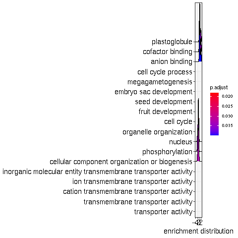
![](ridgeplot.png)
]

.panel[.panel-name[GSEA Plot]
<img src="gseaplot.png" height="425px" class="center" />
]

.panel[
.panel-name[R Code]

```r
## Still working
```
]
]